Any-Order Autoregressive Models (AO-ARM) is a concept of autoregressive models that support a generation of tokens in an arbitrary order. The primal advantage of AO-ARMs over MDMs is an absence of probability factorization.

\(p(x_{1:n}) = \prod_{i=1}^n p(x_{\sigma(i)} \mid x_{\sigma(<i)}),\) where \(\sigma\) is a random permutation of token positions.

This formulation allows models to go beyond left-to-right sampling while keeping the model’s probability function correct. Note that AO-ARMs and basically equivalent to MDMs when sampling one token at a time. During the sampling the permutation \(\sigma\) is usually sampled in advance and do not change during the generation.

Papers:

1. XLNet: Generalized Autoregressive Pretraining for Language Understanding, Google, 2020
2. Autoregressive Diffusion Models, Google, 2021
3. Training and Inference on Any-Order Autoregressive Models the Right Way, Stanford, 2022
4. Your absorbing discrete diffusion secretly models the conditional distributions of clean data, Gaoling, 2025

Masked Diffusion Models (MDM) adapt the diffusion models to text by replacing Gaussian noise with categorical. In the basic form, they corrupt a text by masking a fraction of tokens, thus loosing some information. The fraction increases (linearly in most cases) with respect to timestep \(t\). Therefore, a prior distribution is defined as \(q(x) = \delta(x = [M])\). The forward (noising) process is defined through a transition matrix \(Q\) of size \((m+1) \times (m+1)\): \(Q_i = (1 - \beta_i) I + \beta_i \mathbf{1}e_m^{\top}\). This matrix defines the state transition between \([s(i), t(i)]\), where \(s(i) = \frac{i - 1}{T}, t(i) = \frac{i}{T}\).

We can also define a one-step sampling of \(x_{t(i)}\).

where \(\bar{Q}_i = \prod_{j = 1}^i Q_j = \alpha_i I + (1 - \alpha_i)\mathbf{1}e_m^{\top}\) for \(\alpha_i = \prod_{j = 1}^i (1 - \beta_j)\).

Another important way of looking at MDMs is through Kolmogorov equations.

Kolmogorov equations

Let \(p_{ij}(t) = p(x_t = j | x_0 = i)\) be a probability of transitioning from state \(i\) to state \(j\) within a time period \(t\). \(p_{ij}(t)\) satisfy the following properties:

1. Probability: \(p_{ij}(t) \ge 0, \; \sum_{j} p_{ij} = 1 \;\; \forall i, j\)
2. Stationarity: \(p_{ij}(0) = \delta_{ij} = \begin{cases} 1, & i = j,\\ 0, & i \neq j\end{cases}\)
3. Markov property: \(p_{ij}(t + s) = \sum_{k} p_{ik}(t)p_{kj}(s)\)
4. Stochastic continuity: \(p(\)|\(x_{t+h} - x_t\)|\(> \varepsilon) \to 0\) or \(\lim_{t \to 0} p_{ij}(t) = 0\)

Let the following limit exist: \(q_{ij} = \lim_{h \to 0} \frac{p_{ij}(h) - \delta_{ij}}{h}\)

It is easy to see that \(\sum_{k} q_{ik} = 0\). Indeed,

Also let \(p_{ij}(t)\) be differentiable. Then,

This equation is called the Kolmogorov forward equation and it can be derived from the Markov property of \(p_{ij}(t)\).

This reads as the rate of the probability change from one state to another for a particular time \(t\) is equal to the sum of transition probabilities to all states at that time multiplies by the instant probability change rate. So, to calculate how fast does probability change, we accumulate the weighted speeds of probability change for all possible paths.

Matrix exponentials

All these facts can be written with a matrix notation.

Let \(P(t) = \left\{ p_{ij}(t) \right\}_{i,j}\) to be a transition (stochastic) matrix and \(Q = \left\{ q_{ij} \right\}_{i,j}\) to be a transition rate matrix. Then \(P'(t) = P(t) Q\).

Note that we’ve got the simplest separable ordinary differential equation with a known solution in a form of \(P(t) = C \exp(tQ)\). Given that \(P(0) = I\), we derive

One of the main problems of Masked Diffusion Models is that the probability of the original token sequence is factorised: \(p(x^{1:n} \mid x_t^{1:n}) = \prod_{i=1}^n p(x^i \mid x_t^{1:n})\). This assumption leads to incorrect sampling when multiple tokens are sampled at one step, as they are treated independently by the model.

Multiple papers propose different strategies to mitigate this issue:

1. Self-Speculative Masked Diffusions, DeepMind, 2025

Text generation requires a Language Model to produce a grammatically correct coherent text. Text generation might be unconditionan (unrestricted) and conditional (the text must meet a certain condition). Both generation types have their limitations and benefits.

Unconditional generation

Unconditional text generation isn’t very useful on its own for most real-world tasks. That’s because generated text usually needs to follow certain rules—like keeping the meaning when translating into another language or giving a question-related answer when asked a question.

Nevertheless, unconditional generation does not require a labeled dataset. Thus, the model can be trained using any text data sourced from the internet. This feature essentially eliminates restrictions on the amount of training data, allowing for the creation of powerful Large Language Models (LLMs).

Even though LLMs trained this way might not be useful right away, they can be fine-tuned for specific tasks using smaller, labeled datasets. They can also do surprisingly well at new tasks without any training—or with just a few examples—in zero-shot or few-shot learning paradigm [1]. That is why unconditional generation is the base for all modern language models.

Conditional generation

Conditional generation is more challenging to implement, as the model must process an additional input—the condition—in order to follow it correctly. Modern transformer-based architectures [2] handle this in different ways: Encoder-Decoder models use an additional encoder to process the condition and pass it to the decoder via cross-attention, while Decoder-only models typically concatenate the conditional text with the target sequence. Note that the latter approach isn’t applicable to multimodal text generation—for example, generating image captions.

Model types

In the current state of the field, the dominating text generation model is autoregressive Transformer Decoder-only LLM. However, other approaches also exist.

• LSTM is an outdated approach that is being tried to find a new application [3].
• State Space Models (SSM) are trying to speed up the transformer by abandoning the quadratic time mechanism of attention [4].
• Diffusion models are the current SOTA in image generation that is being adapted for text generation [5, 6].

Datasets and Benchmarks

Unconditional generation:

• WikiText: a collection of over 100 million tokens (~0.5GB) extracted from the set of verified Good and Featured articles on Wikipedia.
• OpenWebText: Unofficial open-source recreation of OpenAI’s WebText (~40GB).
• The Pile: a massive, diverse dataset (~800GB) including books, web pages, GitHub, and academic papers.
• BooksCorpus: collection of books of various genres scraped from the indie ebook distribution website Smashwords. Used for pretraining BERT and GPT (~5GB).
• Common Crawl: a massive crawl of the web (~9.5PB); used to train GPT, LLaMA, etc. Needs a lot of cleaning.
• C4: a colossal, cleaned version of Common Crawl dataset developed by Google and Meta (~750GB). C4 was created by taking a single month’s scrape of Common Crawl and removing duplicate, placeholder, nonsensical and non-English language content. It was used for training T5, LaMDA, LLaMA and other models.
• Project Gutenberg: a set of public domain books (~15GB). Good for literary language modeling.

Conditional generation:

Condition generation has various practical apptications: machine translation, summarization, detoxification, paraphrasing, text simplification, question answering and so on. Each of such tasks has several dedicated datasets.

• Machine translation: WMT (Various Years), IWSLT
• Summarization: CNN/Daily Mail, XSum
• Detoxification: Paradetox
• Paraphrasing: Quora Question Pairs, PAWS
• Text simplification: ASSET, Wiki-Auto, WikiSplit
• Question answering: SQuAD, MS MARCO

As modern models become more powerful, these datasets are no longer complex enough to compare models with each other. Moreover, for a more to add more context to model performance, it became necessary to measure the quality of models on a wide range of tasks at once. That is how specialized benchmarks were developed.

General Language Understanding

• GLUE (General Language Understanding Evaluation) – text classification benchmark.
• SuperGLUE – harder version of GLUE for advanced models, evaluates coreference and reasoning.
• MMLU (Massive Multitask Language Understanding) – evaluates ability to answer questions about math, law, medicine and so on.
• HellaSwag – evaluates the commonsense knowledge by testing the ability to predict most plausible sentence ending.
• GPQA – a multiple-choice, Q&A dataset of very hard questions written and validated by experts in biology, physics, and chemistry.

Factuality and Truthfulness

• TruthfulQA – questions that test truthfulness and common misconceptions.
• FEVER – fact-checking based on Wikipedia evidence.

Multilingual Q&A

• MMMLU (Multilingual Massive Multitask Language Understanding) – evaluates ability to answer questions in multiple languages.

Retrieval-Augmented Generation

• TriviaQA – general knowledge questions.
• Natural Questions – open-ended questions from Google search.

Coding

• SWE-bench Verified – evaluates ability to solve GitHub software issues.
• Terminal-Bench – tests AI agents in real terminal environments.
• HumanEval – measures functional correctness for synthesizing programs from docstrings.

References

[1] Jason Wei et al. Finetuned Language Models are Zero-Shot Learners. ICLR 2022. https://openreview.net/forum?id=gEZrGCozdqR.
[2] Ashish Vaswani et al. Attention is all you need. NeurIPS 2017. https://papers.nips.cc/paper_files/paper/2017/hash/3f5ee243547dee91fbd053c1c4a845aa-Abstract.html.
[3] Maximilian Beck et al. xLSTM: Extended Long Short-Term Memory. NeurIPS 2024, https://openreview.net/forum?id=ARAxPPIAhq.
[4] Albert Gu et al. Efficiently Modeling Long Sequences with Structured State Spaces. ICLR 2022. https://openreview.net/forum?id=uYLFoz1vlAC.
[5] Jacob Austin et al. Structured Denoising Diffusion Models in Discrete State-Spaces, NeurIPS 2021. https://papers.neurips.cc/paper/2021/hash/958c530554f78bcd8e97125b70e6973d-Abstract.html.
[6] Xiang Lisa Li et al. Diffusion-LM Improves Controllable Text Generation. NeurIPS 2022. https://openreview.net/forum?id=3s9IrEsjLyk.

Text retrieval is a language modelling task, which goal is to find relevant information stored as text, such as documents or articles, in response to a user’s query. It involves matching a query (a question, keywords, or text) against a set of text documents and returning the most relevant ones. This process is crucial for various applications like search engines, question answering systems, and document retrieval in legal, medical or any other field.

Dense Retrieval: Pretrained language models (PLMs) are used to generate dense vectors (embeddings) that capture the semantic meaning of text, enabling more accurate semantic matching. Learning-based Ranking: Models are trained to learn relevance scores and rank documents accordingly.

Model types

The whole concept of text retrieval in built on idea of representing a text with a real-numbered vector (embedding) of fixed length. Then, text similarity can be measured as a proximity of the corresponding vectors [1].

The first attempts represented texts using bag-of-words or tf-idf sparce vectors [2]. Based on this scheme, the relevance can be estimated according to the lexical similarity between sparse query and text vectors. Such relevance computation resulted in a poor retrieval quality as it doesn’t account for text semantics directly.

Since the invention of the Transformer model, BERT-based approaches have largely raised text retrieval quality bar. There are two different types of retrieval models: dual-encoder and cross-encoder. Dual-encoder retrieval methods compute embeddings for query and all documents separately and then measure the distance between embeddings, while cross-encoder methods compute a single similarity score for each $\langle$query, document$\rangle$ pair (BERT receives two texts separated with [SEP] token). The former approach it preferable when the list of candidate documents is large, because embeddings for all documents can be pre-computed, which increases the indexing speed. The latter method works better when the amount of documents is small, because it measures relevance better due to the lack of need for information compression.

Also, in the recent years, LLMs started being applied for text retrieval. As LLMs are created only for text generation, the retrieval is done by prompting. For example,

Rate the semantic similarity between the following two sentences on a scale from 0 to 5, where 0 means completely different and 5 means identical in meaning.

Sentence 1: A man is riding a bicycle.
Sentence 2: A person is biking on the road.

Answer (0-5):

Benchmarks

There are not that much benchmarks for evaluating retrieval capabilities of language models as there are for testing language understanding. However, each benchmark covers many aspects of retrieval problem.

• BEIR – 20+ information retrieval datasets (e.g., TREC, SciFact, FEVER)
• MS-MARCO – Microsoft benchmark focused on passage ranking for search relevance.
• HotpotQA – multi-hop question answering with reasoning across documents.
• Natural Questions (NQ) – open-domain QA from Google search with a query, a long answer and a target short answer.
• MTEB (Massive Text Embedding Benchmark) – benchmark with over 50 datasets across 8 NLP task types. Designed primarily for evaluating sentence and document embeddings, like those produced by SBERT, OpenAI embeddings, GTE, or Cohere models.

References

[1] Wayne Xin Zhao et al. Dense Text Retrieval Based on Pretrained Language Models: A Survey. 2024. https://arxiv.org/abs/2211.14876.
[2] G. Salton et al. A vector space model for automatic indexing. 1975. https://dl.acm.org/doi/pdf/10.1145/361219.361220.

Link to the paper

TL;DR: Text AutoEncoder pre-trained on unsupervised denoising task to generalize on downstream text classification. Paper provides a lot of context by comparing many text embedding methods on heterogeneous domains.

Idea

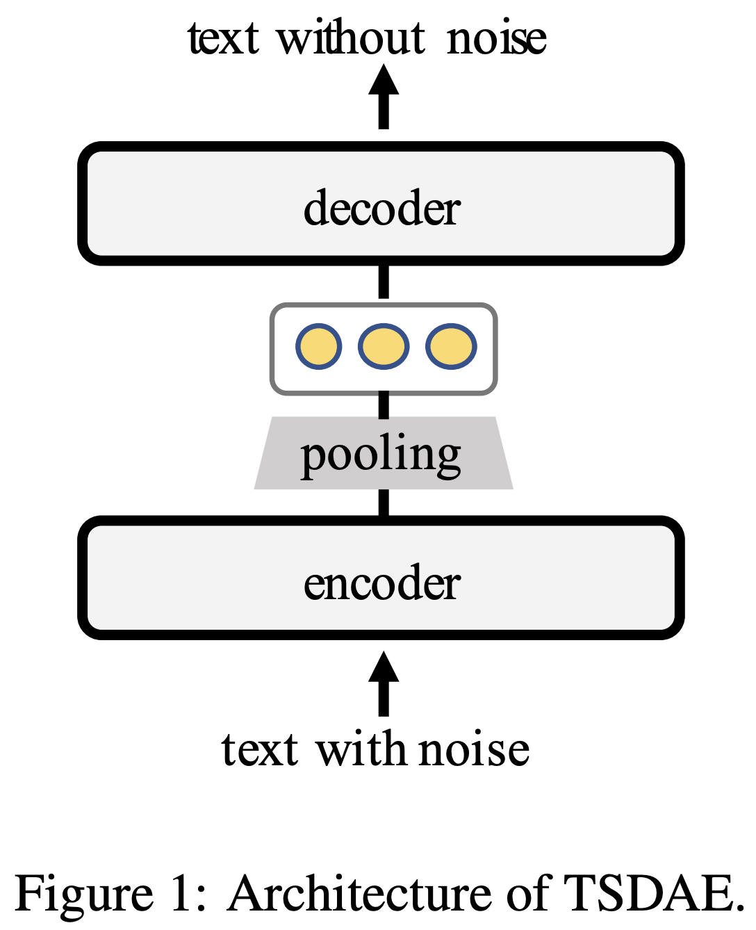
Authors aim to train a model in unsupervised or semi-supervised manner to extract meaningful text embeddings. In order to do it, they build an encoder-decoder architecture similar to Transformer to reconstruct an input text. However, unlike Transformer, the decoder has as access only to a single text embedding extracted by the encoder in the form of the output of the [CLS] token. Additionally, authors corrupt an input text by deleting 60% of tokens.

Experimental setup

Arguing that the previously reported performance on STS () dataset poorly correlate with the performance real-world tasks, authors compare TSDAE to other methods on AskUbuntu (Re-Ranking), CQADupStack (Information Retrieval), TwitterPara (Paraphrase Identification), and SciDocs (Re-Ranking) datasets. In all tasks, the model is required to measure the similarity between an input query and a set of candidates. The paper utilize cosine similarity between text embeddings.

Training setup

The TSDAE approach is tested in three settings: unsupervised learning, domain Adaptation and pre-training.

• Unsupervised Learning: model have access only to unlabeled sentences from the target task.
• Domain adaptation: model have access to unlabeled sentences from the target task and labeled sentences from NLI and STS benchmark. Two setups were tested: 1) training on NLI+STS data, then unsupervised training to the target domain, 2) unsupervised training on the target domain, then supervised training on NLI + STS.
• Pre-Training: model have access to a larger collection of unlabeled sentences from the target task and a smaller set of labeled sentences from the target task.

Baselines

TSDAE is compared to various approaches.

Pre-trained Transformer-based unsupervised methods:

• MLM (Masked-Language-Model): mean pooling over the BERT output token embeddings.
• CT (Contrastive Tension) finetunes pre-trained Transformers in a contrastive-learning fashion. Views the identical sentences as the positive examples. Uses two models with the same initial parameters to encode first and second texts respectively.
• SimCSE: same as CT, but applies different dropout masks for the same sentence and uses single model.
• BERT-flow freezes BERT weights and pushes token embeddings close to a standard Gaussian distribution. The text embeddings is obtained by pooling over processed token embeddings.

Other unsupervised approaches:

• BM25: term-matching method without trainable parameters.
• GloVe: mean pooling over the GloVe embeddings trained on a large corpus from the general domain.
• Sent2Vec: similar to GloVe model trained on the in-domain unlabeled corpus.
• BERT-base-uncased with mean pooling.

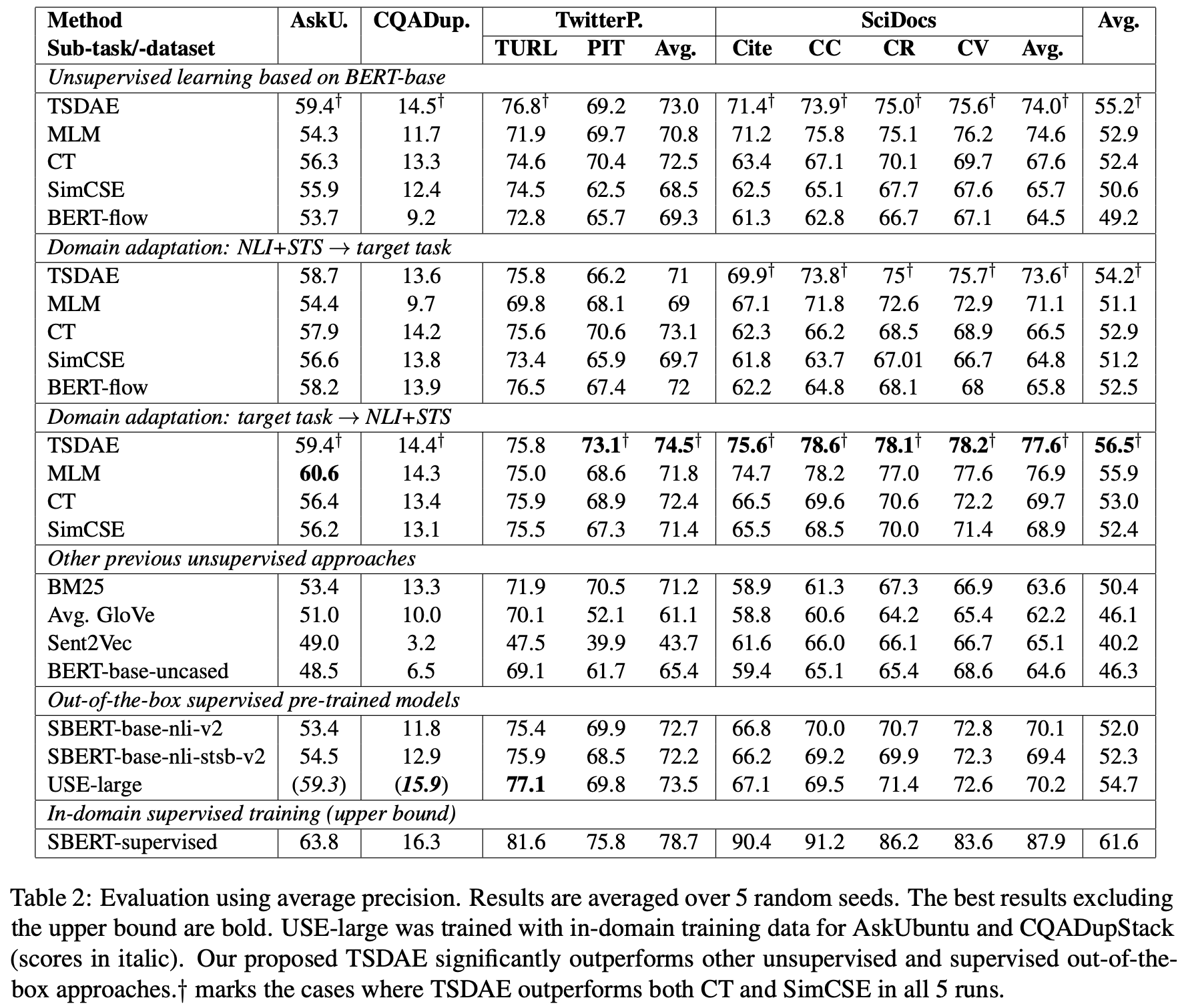
Results

The comparison results are presenter in the table below. Interestingly, a simple MLM approach scores higher than other specialized methods in most setups. Also, in domain adaptation setting, first training on the target domain, and then training with labeled NLI+STS achieves better results than the opposite direction. Overall, TSDAE shows the best results over all datasets.

Link to the paper

TL;DR: Gaussian Diffusion Model trained end-to-end on word embeddings.

Diffusion process

The first step in building a diffusion is to convert text into continuous data sample. Authors do it by learning embeddings for each token in a vocabulary.

where \(\mathbf{w}\) is a sequence of input tokens.

After that \(x_0\) is sampled from the distribution \(q_\phi(\mathbf{x}_0 \mid \mathbf{w})=\mathcal{N}\left(\operatorname{Emb}(\mathbf{w}), \sigma_0 I\right)\), where \(\sigma_0 = 0.0001\).
Alexander’s remark: authors do not explain the necessity of \(\sigma_0\) to be greater than 0 and the chosen value makes \(x_0\) indistinguishable from \(\operatorname{Emb}(\mathbf{w})\).

After defining \(x_0\) the forward process can be written as a common gaussian diffusion process.

The goal is to learn a model to approximate a reverse (denoising) process

One more crucial step in the conversion of generated \(x_0\) into tokens \(\mathbf{w}\). Authors call this step rounding and parametrize it by the trainable model \(p_\theta\left(\mathbf{w} \mid \mathbf{x}_0\right)=\prod_{i=1}^n p_\theta(w_i \mid x_i)\). In practice, it is implemented as a single linear layer \(p_\theta(. \mid x_i) = \operatorname{softmax}(Wx_i)\).

The resulting pipeline can be depicted like this.

Training objective

The diffusion model and embeddings are trained simultaneously by minimizing the following loss function

Alexander’s remark: In the official implementation the term \(\left\|f_\theta(\mathbf{x}_t, t) - \mathbf{x}_0\right\|^2\) is replaced with \(\left\|\mu_\theta\left(\mathbf{x}_t, t\right) - \hat{\mu}\left(\mathbf{x}_t, \mathbf{x}_0\right)\right\|^2\), where \(\mu_\theta\left(\mathbf{x}_t, t\right)\) is a mean of the posterior distribution \(q(x_{t-1} | x_t)\) calculated using the predicted \(x_0\). While these objectives are almost identical in terms of an optimal solution, they have different scaling constants, which might be important. In addition, authors also add a regularization loss term \(\left\|\sqrt{\bar{\alpha}_T}x_0\right\|^2\). Without this term embeddings most probably will explode, because it makes the denoising task trivial (SNR becomes huge for all timesteps).

The term \(-\log p_\theta(\mathbf{w} \mid \mathbf{x}_0)\) is required to prevent another unwanted local minimum – embedding collapse.

Important. Trained embeddings turns out to be better, than fixed pre-trained. Also, learning to predict \(x_0\) results in much better quality, than predicting \(\varepsilon\) as commonly done in image diffusion models.

Clamping trick

During the generation process, authors replace the predicted \(x_0\) with the closest embedding.

They call this method clamping trick and claim that it increase the generation quality by forcing a model to commit to a particular token for intermediate diffusion steps.

Controllable Text Generation

Controllable text generation is equivalent ot sampling from the distribution

where \(p\left(\mathbf{x}_{t-1} \mid \mathbf{x}_t, \mathbf{c}\right) \propto p\left(\mathbf{x}_{t-1} \mid \mathbf{x}_t\right) \cdot p\left(\mathbf{c} \mid \mathbf{x}_{t-1}, \mathbf{x}_t\right) = p\left(\mathbf{x}_{t-1} \mid \mathbf{x}_t\right) \cdot p\left(\mathbf{c} \mid \mathbf{x}_{t-1}\right)\)

After each diffusion step authors run 3 updates on \(\mathbf{x}_{t-1}\) moving it in the direction of the following gradient with Agagrad

where \(\lambda\) is a hyperparameter that allows to control fluency. \(\log p(\mathbf{c} \mid \mathbf{x}_{t-1})\) is evaluated using a pre-trained classifier.

To compensate for the generation speed authors use \(T = 200\) for controllable text generation instead of default \(T = 2000\).

Minimum Bayes Risk Decoding

In order to decrease the variance in generated texts and increase overall quality, authors apply Minimum Bayes Risk (MBR) decoding for controlled generation tasks.

They generate a set of texts \(\mathcal{S}\) and chose one with minimal expected risk.

where \(\mathcal{L}\) is a negative BLEU score.

Alexander’s remark: This is a kind of cheat, because the technique produces samples of better quality in exchange for a loss of computing speed. This loss of speed should be taken into account, as it limits the practical applicability. Additionally, the use of MBR makes it harder to compare Diffusion LM with other approaches, and it suggests that without MBR the quality of the proposed method drops significantly.

Datasets

The evaluation is conducted using two datasets: E2E (50k restaurant reviews) and ROCStories (98k simple five-sentence stories).

Control tasks

Authors consider 6 control tasks shown in this table. The first 4 tasks rely on a classifier, and the last 2 tasks are classifier free.

Results

Link to the paper

TL;DR: Continuous diffusion with cross-entropy loss, trainable embeddings and time warping.

Idea

The diffusion operates in the space of token embeddings. For training the cross-entropy loss is used as it is allows to train embeddings with diffusion model. Time warping is used to automatically control the distribution of model capacity across the noise levels.

Score interpolation

Diffusion models are typically trained by minimising the score matching objective (MSE).

where \(x\) is the noised sample and \(t\) is the timestep. Authors replace it with cross-entropy loss using probabilistic prediction of the clean sample \(x_0\).

where \(w\) is an input token and \(e_w\) is the embedding of the \(w\)th token in the vocabulary.

Score function estimate is obtained by linearly interpolating all possible values with predicted probabilities.

where \(V\) is the size of the vocabulary.

Authors choose the following probability flow ODE for the diffusion model: \(dx = −t \nabla_x \log p_t(x) dt\). In this formulation, \(t\) corresponds directly to the standard deviation of the Gaussian noise that is added to \(x_0\) to simulate samples from \(p_t(x)\).

Due to the fact that \(p_t(x)\) is a Gaussian distribution,

Therefore,

This allows to approximate the score function using the trained model \(p_{\theta}\) and estimating the ground truth embedding vector as \(\mathbb{E}_{p(x_0 \mid x, t)}[x_0] \approx \hat{x}_0 = \sum_{i=1}^V p_{\theta}(x_0 = e_i \mid x, t) \cdot e_i\).

Diffusion on embeddings

The choice of CE loss allows authors to train embeddings simultaneously with the diffusion model, because with score matching (MSE) loss embeddings would result in collapse of the embedding space. To prevent the embeddings explosion, authors L2-normalize embeddings before the use. They also normalize the predictions of \(x_0\) on every denoising step to match the unit norm.

Alexander’s remark: L2-normalization might be tricky. While it keeps the embeddings norm fixed, this method may force embeddings to accumulating all information in a small subset of vector coordinates and zeroing the rest of coordinates, which is not a desired behaviour.

Time warping (important idea)

The diffusion model share its parameters between all noise levels. This means that during the training the model somehow distributes its capacity between different noise levels. To control this distribution, we can adjust the weights of loss terms for different noise levels or tune the noise scheduler. Authors state that the entropy of the model predictions should increase linearly with the growth of \(t\). Therefore, during the generation the uncertainty of the model predictions (or the amount of information that is recovered by model) should change at a constant rate.

In order to embed this idea to the model, authors introduce the cumulative distribution function (CDF) \(F\) and sample \(t\) by first sampling \(u \sim U[0, 1]\) and then computing \(t\) as \(t = F^{-1}(u)\).

In practice, authors fit an unnormalised monotonic function \(\tilde{F}(t)\) to the observed cross-entropy loss values \(L(t)\). Cross-entropy loss values here estimate the prediction entropy.

\(\tilde{F}(t)\) is parametrised as a monotonic piecewise linear function, which is very straightforward to normalise and invert.

Ablation shows that time warping significantly increase the generation quality in terms of perplexity.

Conditional generation

For conditional generation authors keep the conditioning tokens clean during the training and add noise only to tokens which should be generated. Also, model receives a binary mask indicating which tokens are clean and which are noisy. Authors experiment with tree masking setups: prefix masking (the sequence prefix of random length is kept clean), random masking (completely random tokens are kept clean) and combination of both. Surprisingly, they found out, that the combination of masking schemes lead to the best prefix completion performance.

During the generation self-conditioning and classifier-free guidance are also applied. Both significantly boost the performance.

Results

The paper provides a very detailed ablation study of all described methods. However, there is no comparison with other diffusion methods. The comparison with autoregressive transformer on the machine translation task shows that the CDCD performs worse even with 100 samples used for Minimum Bayes-Risk decoding.

Continuous Diffusion Models for text generation is an attempt to adapt diffusion models (SOTA for image generation) to text data. Unlike Discrete Diffusion Models, continuous diffusion models do not change the noising process (although there are exceptions). Instead they map discrete text into a continuous latent space and run a default diffusion process there.

Formally speaking, let \(w = (w_1, \dots, w_n)\) be an input sequence of tokens of size \(n\). Then its latent \(x_0 \in \mathbb{R}^{m \times d}\) can be obtained using encoder model \(E\), \(x_0 = E(w)\). Note that after the mapping the length of the sequence might change (\(m \neq n\)). Each noised latent \(x_t\) for \(t \in [1, T]\) is sampled from the Gaussian distribution, \(x_t \sim \mathcal{N}(\gamma_t x_0, \sigma_t^2I)\), where \(\gamma_t\) and \(\sigma_t\) are hyperparameters that control the noise injection speed, such that \(\forall s < t, \gamma_s > \gamma_t\) and \(\sigma_s < \sigma_t\) and \(\gamma_T = \sigma_1 = 0, \gamma_0 = \sigma_T = 1\).

During the training a diffusion model \(f_\theta\) learns to reconstruct an original latent \(x_0\) based on its noised version \(x_t\). The generation is performed by starting from the pure noise \(x_T\) and then iteratively refining it using the trained diffusion model \(f_\theta\) until \(\hat{x}_0\) is recovered. At the end of the generation process, decoder \(D\) converts generated latent \(\hat{x}_0\) back to tokens, \(\hat{w} = D(\hat{x}_0)\).

Most commonly encoder \(E\) simply maps each token into its embedding vector, so \(m = n\). Decoder \(D\) then converts generated embedding to a token corresponding to a closes embedding.

At the training phase the main loss term which is optimized is the MSE between the original latent \(x_0\) and the predicted latent.

where \(f_\theta\) is a diffusion model that is being trained.

Often embeddings are optimized simultaneously with the diffusion model. Then some additional loss terms must be added in order to prevent the collapse of the embeddings space.

Note that if a diffusion model is trained with cross-entropy loss instead of MSE, embeddings will explode and this problem must also be fixed. For example, by normalizing embeddings before each use as in CDCD method.

Language Modelling is the process of developing a statistical or machine learning model that can understand, generate, or predict language—usually natural language like English.

Examples of Language Models:

• Encoder-Decoder (Sequence-to-sequence): Transformer, T5, BART, …
• Decoder (Text generation): RNN, LSTM, GPT, LLaMA, Claude, Mistral, …
• Encoder (Text classification, Text embedding): BERT, RoBERTa, E5, …
• Diffusion models (Text generation): based on Encoder; Diffusion-LM, SEDD, LD4LG, …