Continuous diffusion for categorical data

Link to the paper

TL;DR: Continuous diffusion with cross-entropy loss, trainable embeddings and time warping.

Idea

The diffusion operates in the space of token embeddings. For training the cross-entropy loss is used as it is allows to train embeddings with diffusion model. Time warping is used to automatically control the distribution of model capacity across the noise levels.

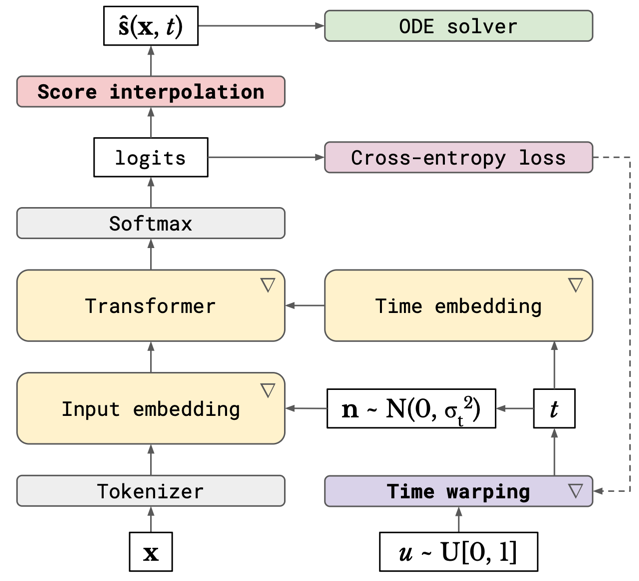
Score interpolation

Diffusion models are typically trained by minimising the score matching objective (MSE).

\[L(\theta) = \mathbb{E}_{t, x} \big[\|s_{\theta}(x, t) - \nabla_x \log p_t(x)\|^2\big],\]

where \(x\) is the noised sample and \(t\) is the timestep. Authors replace it with cross-entropy loss using probabilistic prediction of the clean sample \(x_0\).

\[L(\theta) = -\mathbb{E}_{w, t, x} \big[\log p_{\theta}(x_0 = e_{w} \mid x, t)\big],\]

where \(w\) is an input token and \(e_w\) is the embedding of the \(w\)th token in the vocabulary.

Score function estimate is obtained by linearly interpolating all possible values with predicted probabilities.

\[\hat{s}(x, t) = \sum_{i=1}^{V} p(x_0 = e_i \mid x, t) s(x, t \mid x_0 = e_i) = \mathbb{E}_{p(x_0 \mid x, t)} s(x, t \mid x_0),\]

where \(V\) is the size of the vocabulary.

Authors choose the following probability flow ODE for the diffusion model: \(dx = −t \nabla_x \log p_t(x) dt\). In this formulation, \(t\) corresponds directly to the standard deviation of the Gaussian noise that is added to \(x_0\) to simulate samples from \(p_t(x)\).

Due to the fact that \(p_t(x)\) is a Gaussian distribution,

\[s(x, t \mid x_0) = \nabla_x \log p_t(x \mid x_0) = \frac{x_0 - x}{t^2}\]

Therefore,

\[\hat{s}(x, t \mid x_0) = \frac{\mathbb{E}_{p(x_0 \mid x, t)} [x_0] - x}{t^2}\]

This allows to approximate the score function using the trained model \(p_{\theta}\) and estimating the ground truth embedding vector as \(\mathbb{E}_{p(x_0 \mid x, t)}[x_0] \approx \hat{x}_0 = \sum_{i=1}^V p_{\theta}(x_0 = e_i \mid x, t) \cdot e_i\).

Diffusion on embeddings

The choice of CE loss allows authors to train embeddings simultaneously with the diffusion model, because with score matching (MSE) loss embeddings would result in collapse of the embedding space. To prevent the embeddings explosion, authors L2-normalize embeddings before the use. They also normalize the predictions of \(x_0\) on every denoising step to match the unit norm.

Alexander’s remark: L2-normalization might be tricky. While it keeps the embeddings norm fixed, this method may force embeddings to accumulating all information in a small subset of vector coordinates and zeroing the rest of coordinates, which is not a desired behaviour.

Time warping (important idea)

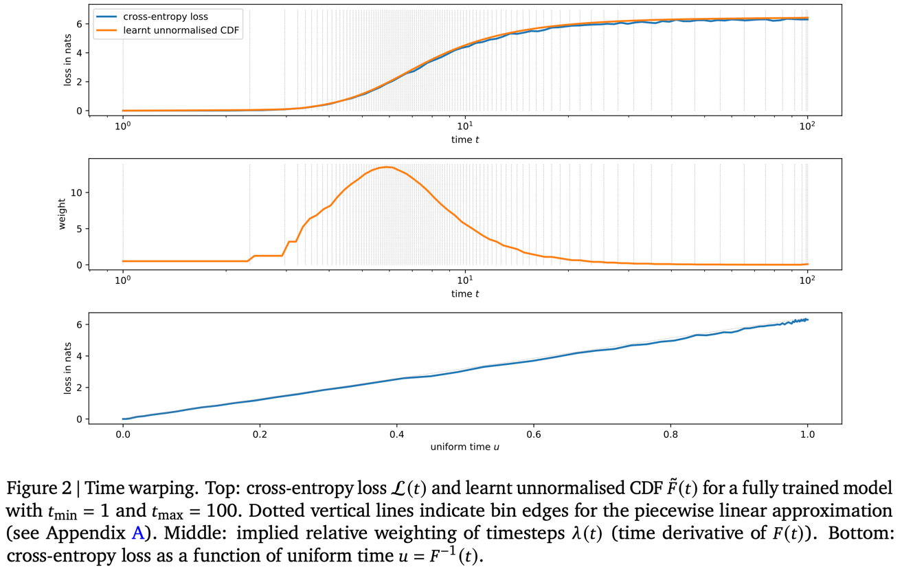
The diffusion model share its parameters between all noise levels. This means that during the training the model somehow distributes its capacity between different noise levels. To control this distribution, we can adjust the weights of loss terms for different noise levels or tune the noise scheduler. Authors state that the entropy of the model predictions should increase linearly with the growth of \(t\). Therefore, during the generation the uncertainty of the model predictions (or the amount of information that is recovered by model) should change at a constant rate.

In order to embed this idea to the model, authors introduce the cumulative distribution function (CDF) \(F\) and sample \(t\) by first sampling \(u \sim U[0, 1]\) and then computing \(t\) as \(t = F^{-1}(u)\).

In practice, authors fit an unnormalised monotonic function \(\tilde{F}(t)\) to the observed cross-entropy loss values \(L(t)\). Cross-entropy loss values here estimate the prediction entropy.

\[\min(\tilde{F}(t) - L(t))^2\]

\(\tilde{F}(t)\) is parametrised as a monotonic piecewise linear function, which is very straightforward to normalise and invert.

Ablation shows that time warping significantly increase the generation quality in terms of perplexity.

Conditional generation

For conditional generation authors keep the conditioning tokens clean during the training and add noise only to tokens which should be generated. Also, model receives a binary mask indicating which tokens are clean and which are noisy. Authors experiment with tree masking setups: prefix masking (the sequence prefix of random length is kept clean), random masking (completely random tokens are kept clean) and combination of both. Surprisingly, they found out, that the combination of masking schemes lead to the best prefix completion performance.

During the generation self-conditioning and classifier-free guidance are also applied. Both significantly boost the performance.

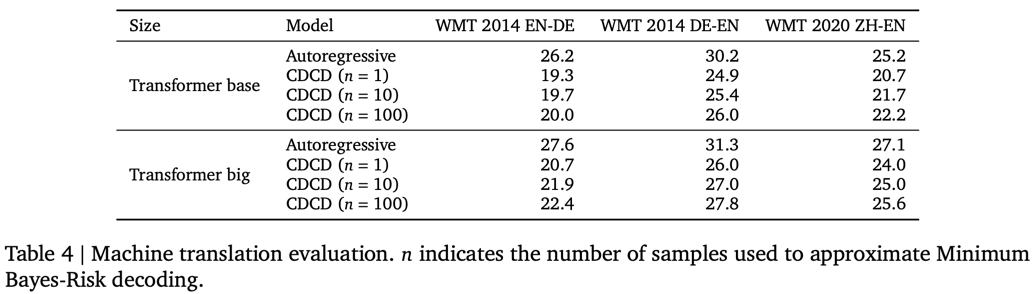
Results

The paper provides a very detailed ablation study of all described methods. However, there is no comparison with other diffusion methods. The comparison with autoregressive transformer on the machine translation task shows that the CDCD performs worse even with 100 samples used for Minimum Bayes-Risk decoding.