Diffusion-LM
TL;DR: Gaussian Diffusion Model trained end-to-end on word embeddings.
Diffusion process
The first step in building a diffusion is to convert text into continuous data sample. Authors do it by learning embeddings for each token in a vocabulary.
\[\operatorname{Emb}(\mathbf{w})=\left[\operatorname{Emb}(w_1), \ldots, \operatorname{Emb}(w_n)\right] \in \mathbb{R}^{n d},\]where \(\mathbf{w}\) is a sequence of input tokens.
After that \(x_0\) is sampled from the distribution \(q_\phi(\mathbf{x}_0 \mid \mathbf{w})=\mathcal{N}\left(\operatorname{Emb}(\mathbf{w}), \sigma_0 I\right)\), where \(\sigma_0 = 0.0001\).
Alexander’s remark: authors do not explain the necessity of \(\sigma_0\) to be greater than 0 and the chosen value makes \(x_0\) indistinguishable from \(\operatorname{Emb}(\mathbf{w})\).
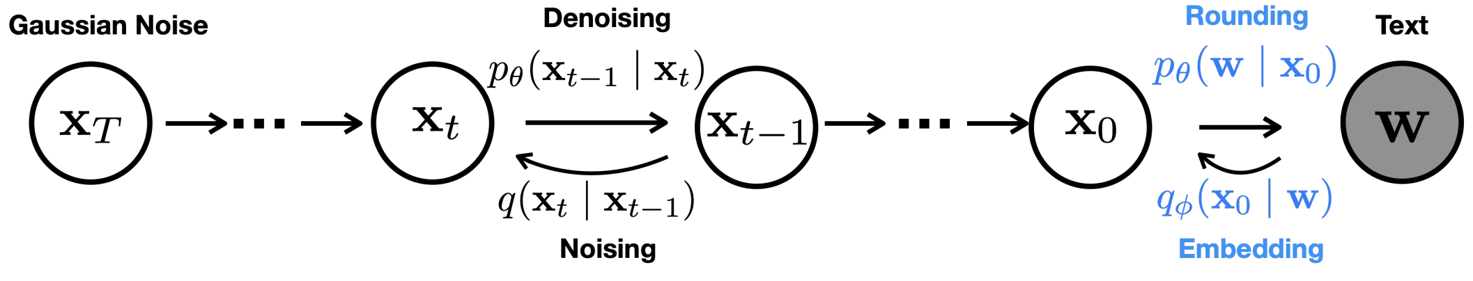
After defining \(x_0\) the forward process can be written as a common gaussian diffusion process.
\[q\left(\mathbf{x}_t \mid \mathbf{x}_{t-1}\right)=\mathcal{N}\left(\mathbf{x}_t ; \sqrt{1-\beta_t} \mathbf{x}_{t-1}, \beta_t \mathbf{I}\right)\]The goal is to learn a model to approximate a reverse (denoising) process
\[p_\theta\left(\mathbf{x}_{t-1} \mid \mathbf{x}_t\right)=\mathcal{N}\left(\mathbf{x}_{t-1} ; \mu_\theta\left(\mathbf{x}_t, t\right), \Sigma_\theta\left(\mathbf{x}_t, t\right)\right)\]One more crucial step in the conversion of generated \(x_0\) into tokens \(\mathbf{w}\). Authors call this step rounding and parametrize it by the trainable model \(p_\theta\left(\mathbf{w} \mid \mathbf{x}_0\right)=\prod_{i=1}^n p_\theta(w_i \mid x_i)\). In practice, it is implemented as a single linear layer \(p_\theta(. \mid x_i) = \operatorname{softmax}(Wx_i)\).
The resulting pipeline can be depicted like this.
Training objective
The diffusion model and embeddings are trained simultaneously by minimizing the following loss function
\[\mathcal{L}^{\mathrm{e}2\mathrm{e}}(\mathbf{w})=\underset{q_\phi\left(\mathbf{x}_{0: T} \mid \mathbf{w}\right)}{\mathbb{E}}\left[\sum_{t=2}^T \left\|f_\theta(\mathbf{x}_t, t) - \mathbf{x}_0\right\|^2 + \left\|\mu_\theta\left(\mathbf{x}_1, 1\right) - \operatorname{Emb}(\mathbf{w})\right\|^2-\log p_\theta\left(\mathbf{w} \mid \mathbf{x}_0\right)\right]\]Alexander’s remark: In the official implementation the term \(\left\|f_\theta(\mathbf{x}_t, t) - \mathbf{x}_0\right\|^2\) is replaced with \(\left\|\mu_\theta\left(\mathbf{x}_t, t\right) - \hat{\mu}\left(\mathbf{x}_t, \mathbf{x}_0\right)\right\|^2\), where \(\mu_\theta\left(\mathbf{x}_t, t\right)\) is a mean of the posterior distribution \(q(x_{t-1} | x_t)\) calculated using the predicted \(x_0\). While these objectives are almost identical in terms of an optimal solution, they have different scaling constants, which might be important. In addition, authors also add a regularization loss term \(\left\|\sqrt{\bar{\alpha}_T}x_0\right\|^2\). Without this term embeddings most probably will explode, because it makes the denoising task trivial (SNR becomes huge for all timesteps).
The term \(-\log p_\theta(\mathbf{w} \mid \mathbf{x}_0)\) is required to prevent another unwanted local minimum – embedding collapse.
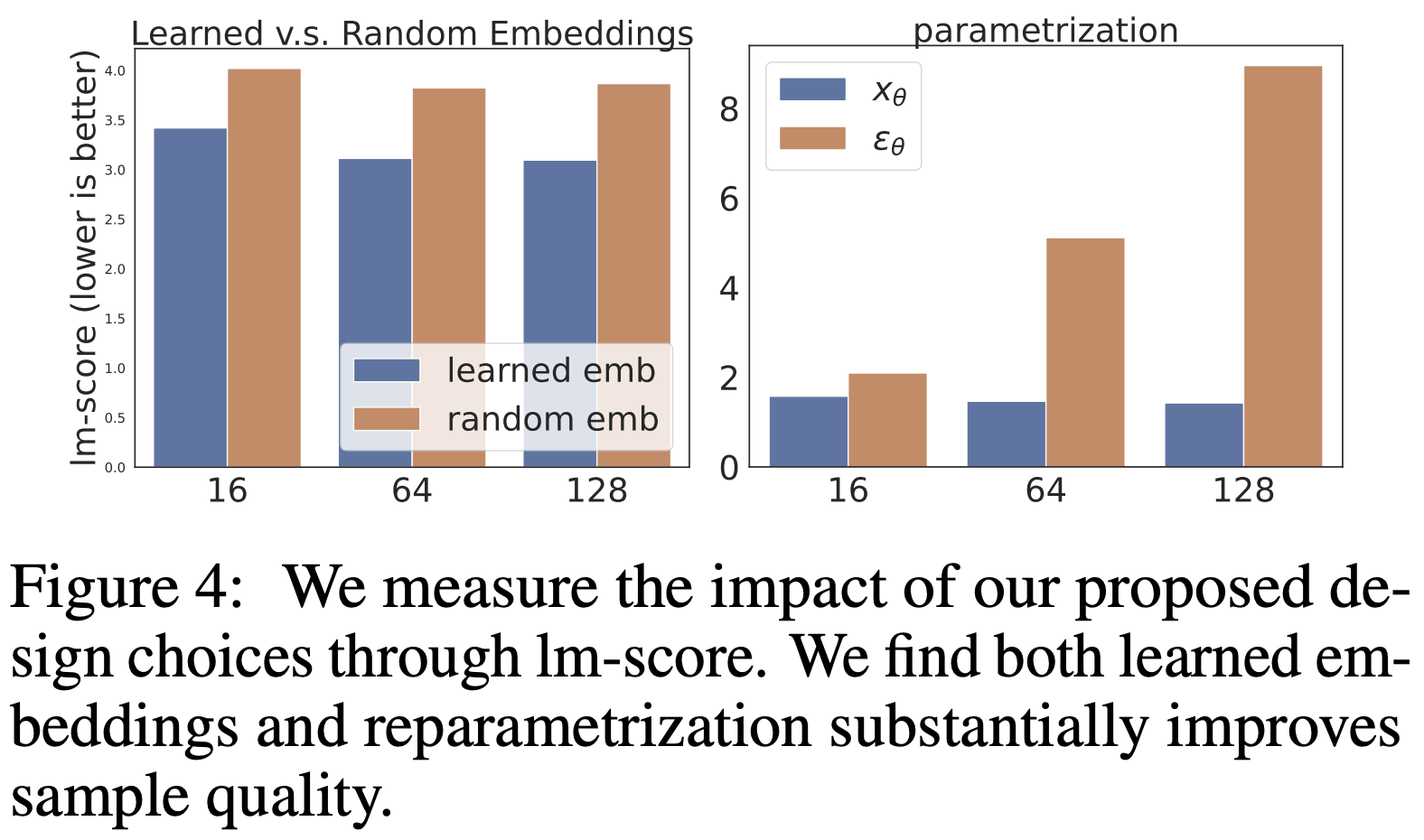
Important. Trained embeddings turns out to be better, than fixed pre-trained. Also, learning to predict \(x_0\) results in much better quality, than predicting \(\varepsilon\) as commonly done in image diffusion models.
Clamping trick
During the generation process, authors replace the predicted \(x_0\) with the closest embedding.
\[\mathbf{x}_{t-1}=\sqrt{\bar{\alpha}_{t-1}} \cdot \operatorname{Clamp}\left(f_\theta\left(\mathbf{x}_t, t\right)\right)+\sqrt{1-\bar{\alpha}_{t-1}} \epsilon\]They call this method clamping trick and claim that it increase the generation quality by forcing a model to commit to a particular token for intermediate diffusion steps.
Controllable Text Generation
Controllable text generation is equivalent ot sampling from the distribution
\[p\left(\mathbf{x}_{0: T} \mid \mathbf{c}\right)=\prod_{t=1}^T p\left(\mathbf{x}_{t-1} \mid \mathbf{x}_t, \mathbf{c}\right),\]where \(p\left(\mathbf{x}_{t-1} \mid \mathbf{x}_t, \mathbf{c}\right) \propto p\left(\mathbf{x}_{t-1} \mid \mathbf{x}_t\right) \cdot p\left(\mathbf{c} \mid \mathbf{x}_{t-1}, \mathbf{x}_t\right) = p\left(\mathbf{x}_{t-1} \mid \mathbf{x}_t\right) \cdot p\left(\mathbf{c} \mid \mathbf{x}_{t-1}\right)\)
After each diffusion step authors run 3 updates on \(\mathbf{x}_{t-1}\) moving it in the direction of the following gradient with Agagrad
\[\nabla_{\mathbf{x}_{t-1}} \lambda \log p(\mathbf{x}_{t-1} \mid \mathbf{x}_t) + \nabla_{\mathbf{x}_{t-1}}\log p(\mathbf{c} \mid \mathbf{x}_{t-1}),\]where \(\lambda\) is a hyperparameter that allows to control fluency. \(\log p(\mathbf{c} \mid \mathbf{x}_{t-1})\) is evaluated using a pre-trained classifier.
To compensate for the generation speed authors use \(T = 200\) for controllable text generation instead of default \(T = 2000\).
Minimum Bayes Risk Decoding
In order to decrease the variance in generated texts and increase overall quality, authors apply Minimum Bayes Risk (MBR) decoding for controlled generation tasks.
They generate a set of texts \(\mathcal{S}\) and chose one with minimal expected risk.
\[\hat{\mathbf{w}} = \operatorname{argmin}_{\mathbf{w} \in \mathcal{S}} \sum_{\mathbf{w}' \in \mathcal{S}} \frac{1}{\mathcal{S}} \mathcal{L}(\mathbf{w}, \mathbf{w}'),\]where \(\mathcal{L}\) is a negative BLEU score.
Alexander’s remark: This is a kind of cheat, because the technique produces samples of better quality in exchange for a loss of computing speed. This loss of speed should be taken into account, as it limits the practical applicability. Additionally, the use of MBR makes it harder to compare Diffusion LM with other approaches, and it suggests that without MBR the quality of the proposed method drops significantly.
Datasets
The evaluation is conducted using two datasets: E2E (50k restaurant reviews) and ROCStories (98k simple five-sentence stories).
Control tasks
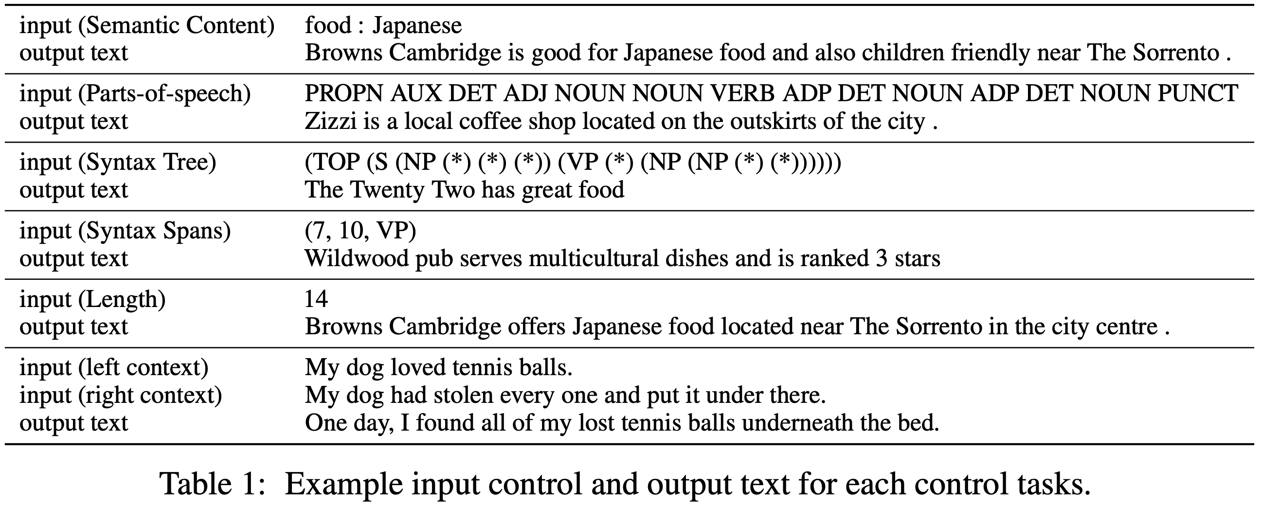
Authors consider 6 control tasks shown in this table. The first 4 tasks rely on a classifier, and the last 2 tasks are classifier free.
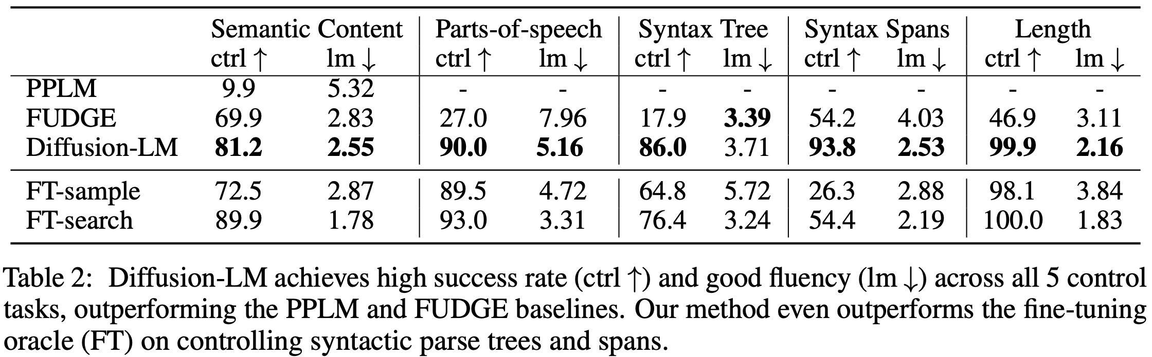
Results